Typical plot of GPS-45 in the open showing Selective Availability. Plot is about 100 x 100 mtrs |
Typical plot with differential correction at same location. Beacon was about 40 km away. Plot is about 4 x 6 mtrs. Grid lines are .00025 deg. |
|
WHAT TO EXPECT |
|
|
|
Typical plot of GPS-45 in the open showing Selective Availability. Plot is about 100 x 100 mtrs |
Typical plot with differential correction at same location. Beacon was about 40 km away. Plot is about 4 x 6 mtrs. Grid lines are .00025 deg. |
|
|

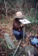
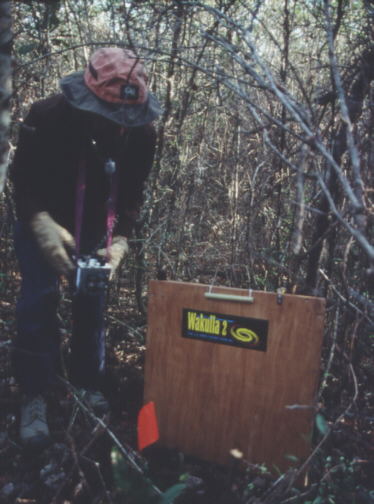
Ground Zero in the Forest |
Differential GPS was used to quickly determine the location of each Radiolocated point to within about 4 meters. The gear could be easily carried and operated by one person. It worked reasonably well under the forest canopy. Originally, we had discussed using conventional land surveying techniques to locate each point relative to the entrance to Wakulla Spring, but it became obvious that it was impractical. We needed the location as soon as possible after each point was located and simply didn't have the manpower to clear the sight lines and man the transit every day or two. The cave spread out over 5 square kilometers with old growth forest in the park and dense ~12 foot scrub in the formerly clearcut woods outside the boundary where a sharp machette was required equipment. |
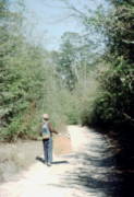
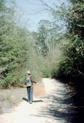
Road thru scrub forest outside the park |
|
|

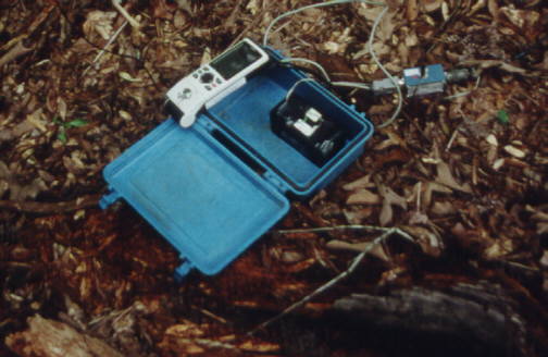
GPS-45, 12V battery, DGPS adapter |
A GPS-45 single channel receiver (circa 1994) was used with an inexpensive Eagle all-in-one manually tuned differential Beacon receiver tuned to the nearest Coast Guard beacon (312 kHz) located 325 km south on Egmont Key near Tampa. A custom cable provided both power and DGPS corrections to the GPS-45. The standard serial port connector was later used to download the track plots to a computer. The Beacon receiver was mounted on a copper grounding pole and shared the battery. |
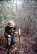
Differential Beacon Receiver and 5 ft whip |
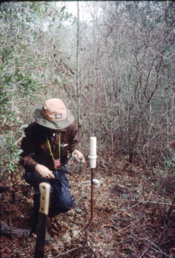
Lowe "mag-mount" amplified GPS antenna on ground plane |
A LOWE "mag-mount" external amplified patch antenna was mounted on a one foot square ground plane and elevated on a pole. In dense scrub as much as 12 ft of pole was used when needed to improve signals and reduce multipath. In a few cases the GPS was set up in a clearing and tied to "Ground Zero" by a single compass and tape survey shot. Typically, at least 300-400 track points would be recorded at 2 sec/pt at each location. The slow "drift" of Selective Availability was not an issue. |
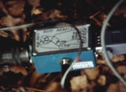
DGPS adapter with 12V battery plug, low voltage LED, serial port Conn. for GPS (incl 12VDC), and "mil" conn. for Beacon receiver. |
|
|
Location A38 outside the park. ~7 x 7 mtrs Nearly as good as open sky (The best plot). |
The points were downloaded and plotted using a Waypoint+, a freeware program that can upload and download tracks and waypoints to Garmin Receivers as well plot in any datum with a cursor calibrated in Lat/Lon or UTM. We used UTM at Wakulla to keep the math simple when plotting or planning. The center of the plot was located by eyeball and the UTM coordinates recorded. This largely eliminated the degradation from multipath. If I had had a receiver that could do fix averaging, I would have used it, but would still have looked at the track plots. Some plots had wild excursions that would throw off the mathematical average, but could usually be saved by eye. |
Location A34 outside the park. ~15 x 15 mtrs with a little multipath from the trees (A typical plot). |
The new points were immediately used to correct the inertial drift of the Wall Mapper to see if the data looked good. It was also plotted on a working Topo Map to determine which overgrown road to chop clear next (outside the park) and where to expect the next Radiolocation signal. They were also plotted in Trimble Survey Office which eventually resulted in a rough outline of the underground passages. In the End, 38 points over Wakulla and nearby Sally Ward Spring (also in the Park) were Radiolocated and given approximate UTM coordinates in this manner. |
Location B17 deep inside the park ~35 x 35 mtrs with serious multipath (The worst plot used). |
Towards the end of the 3 month expedition, all 38 points were
located to within 1 cm using a Trimble GPS plus some transit surveying.
This allowed a real check of the accuracy of DGPS.
The coast Guard gives expected errors as follows: 0.5 meter with a perfect receiver close to the differential beacon plus 1.5 mtrs receiver error plus 1 mtr error for each 150 km from the beacon (325 km at Wakulla) for a total of 4 meters expected error. This is for a ship with a totally clear horizon free of multipath. Our average error for the 38 points was 3.8 meters with the largest error 11.5 mtrs. The median error was 3.5 mtrs. This is very good considering that 2/3 of the points lie inside the park under the old growth trees. Recent experiments with a 12 channel parallel GPS-48 in the woods have resulted in smaller DGPS track plots than the GPS-45, probably because the corrections are applied faster. |
|
|
Open-field non-differential GPS-48 track plot (1024 points) without S/A. Only 4 x 4 meters! The grid .0001 degrees per division |
14 months after Wakulla II ended, Selective Availibility was turned
off for good. This plot, made with a 12 channel parallel receiver hints
that one may now achieve 4 meter accuracy without differential correction!
The eyeball average of this plot gives exactly the same UTM position (1
meter resolution) as the receiver's internal Waypoint averaging function.
The GPS-48 reported a FOM (Figure Of Merit) for this averaged waypoint
of ±13.9 feet (4.2 mtrs). The FOM appears to be a realistic estimate
of actual precision of the fix. The differential data does correct
for ionospheric variations and timing/position errors from each satellite,
but with a plot this small............Current wisdom is that real time
accuracy without S/A is 10 meters horizontal accuracy, one minute of averaging
(1 fix/2 sec) gives 5 meters, and 10 minutes of averaging gives 4 meters.
With DGPS, expect 8 meters without averaging or 3 meters (or better depending
on the GPS receiver and data rate) with 10 minute averaging.
A note for Garmin users: To increase accuracy by averaging (at a fixed location) simply press MARK, select Average, then press ENTER. The FOM will become visible. Do not look at any other screens while averaging! When the FOM has stabilized, simply write down the fix and FOM. It can also be saved as a numbered waypoint (to be renamed later) by selecting Save, then pressing ENTER. In the forest, where the track plot and FOM are larger, it will pay to average for a longer time, perhaps 10-15 minutes. UTM grid coordinates give the best resolution, and are the easiest to plot and work with.. You get 1 meter resolution with UTM, 1.9 meters with DD mm.mmm, and 3.1 meters with DD mm ss.s. |
| This plot is an example of what can be done with differential GPS in the absense of S/A. |